BAFQMC
From local positivity to global symmetry
Bosonic auxiliary-field quantum Monte Carlo
English · 简体中文




Documentation · Get started · The algorithm · Reproduce results · Guide for agents
Worldline and stochastic-series-expansion methods organize sign-free sampling around local matrix-element positivity. BAFQMC establishes nonnegative bosonic weights through global symmetry after Hubbard–Stratonovich decoupling. Reflection positivity (RP) and time-reversal symmetry (TRS) open a new computable region: frustrated bosonic models protected by these symmetries.
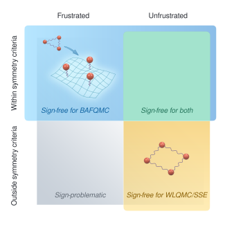
This repository puts the construction to work: finite-temperature solvers for two-flavor bosons on a triangular lattice, with and without onsite pairing; exact diagonalization (ED); and a complete workflow to reproduce the paper's benchmarks. Run new calculations. Extend the method. Build on the code. Everything here is available under MIT.
What can I simulate?
The supplied solvers calculate finite-temperature properties of two boson flavors on a periodic triangular lattice. In the paper's notation, the implemented Hamiltonian is
Here \(U_1\geq0\) is the repulsive relative-density coupling and \(U_2\leq0\) is the attractive total-density coupling. Here \(\hat n_{b,i}=\hat b_i^+\hat b_i\) and \(\hat n_{c,i}=\hat c_i^+\hat c_i\). Simulations use the grand-canonical ensemble \(Z=\mathrm{Tr}e^{-\beta(\hat H-\mu\hat N)}\), with \(\hat N=\sum_i(\hat n_{b,i}+\hat n_{c,i})\). Positive \(t=1\) gives frustrated hopping. The number-conserving solver sets \(\Delta=0\); the Nambu solver supports real onsite pairing.
The lattice has \(N_s=L_xL_y\) sites and primitive vectors
Nearest-neighbor bonds run along \(\mathbf a_1\), \(\mathbf a_2\), and \(\mathbf a_2-\mathbf a_1\), including their reverse directions and periodic images. The benchmarks use \(3\times3\) clusters and measure \(\rho\), \(-E\), \(S_{\mathrm{SF}}(K)\), and \(S_{\mathrm{DW}}(K)\).
You can set the two channels independently: \(U_2=0\) gives the relative-density-only case, while fixing \(U_1=1\) and varying \(U_2\) probes the total-density channel.
The model, lattice, and parameter guide explains the ensemble, HS fields, and reference calculations.
Want to study another model? The model-development guide and dedicated agent skill explain how to extend the lattice, hopping, interactions, and pairing, with matching ED and physics tests.
Work with your agent
If you use a coding agent, give it a request such as one of the following. The agent instructions and task recipes provide the implementation map and verification steps.
Get https://github.com/YinkaiYu/BAFQMC, read AGENTS.md, check the Linux or WSL
prerequisites, build both solvers, and run the small installation tests. Report
the setup path and every check result.
Reproduce every paper benchmark from the default BAFQMC command. Read
AGENTS.md, keep
large raw chains outside Git, retain the processed benchmark data, and report
the resource budget, output paths, and final comparison tables and figures.
Get https://github.com/YinkaiYu/BAFQMC and reproduce all paper benchmarks with
the published parameters and seeds. Save new results in a dedicated directory
and show me the final figures.
I want to study the triangular-lattice model at U1 = 1, U2 = 0, beta = 4 and
mu = -5 while varying the pairing strength. Prepare a separate campaign, check one
small case with ED, and explain the computing budget before production.
Extend the implemented two-channel model to a nearest-neighbor kagome lattice at
t = 1, U1 = 1, U2 = 0, Delta = 0, beta = 4, mu = -5. Read the new-model skill, derive
the HS symmetry, implement the geometry and matching ED and observables,
and validate a small case. Report the computing budget before production.
Add an observable for my research. Derive its estimator using the existing
Green-function convention, implement it in BAFQMC and ED, and verify it on a
small system.
Describe the physics you want to study and the computing resources you can use. Your agent can work through the details in the linked guides.
Reproduce the paper
After environment setup, run:
python3 reproduce.py
This builds the solvers, runs fresh BAFQMC and ED calculations for all 22 benchmark points, processes the measurements, and produces both figures. Allow approximately 12–24 hours, 16 GiB RAM, and 8 GiB free disk on a modern desktop CPU. The default uses one MPI rank and one numerical-library thread, with cases run sequentially. The resource guide gives measured timings and instructions for resuming a campaign.
python3 reproduce.py --plan        # Show the scope and resource estimate
python3 reproduce.py --mode smoke  # Small BAFQMC + ED installation check
Small processed benchmark data, including means and standard errors, are included. Large simulation outputs are generated locally and excluded from Git.
Explore
- Get started: install, run, and find your results.
- Algorithm and conventions: models, symmetry, and observables.
- Output observables: operator definitions and file conventions.
- Extend to other models: from Hamiltonian to tested implementation.
- Research tasks for agents: new calculations and extensions.
- Benchmark details: parameters, data, and reproduction modes.
- Contributing: develop and validate changes.
Paper
Yin-Kai Yu, Zhong-Chao Wei, and Zi-Xiang Li, Sign-problem-free Bosonic Auxiliary Field Quantum Monte Carlo, arXiv:2610.31541 (2026).
If you use BAFQMC in your research, please cite:
@misc{yu2026signproblemfree,
  title         = {Sign-problem-free Bosonic Auxiliary Field Quantum Monte Carlo},
  author        = {Yin-Kai Yu and Zhong-Chao Wei and Zi-Xiang Li},
  year          = {2026},
  eprint        = {2610.31541},
  archivePrefix = {arXiv},
  primaryClass  = {cond-mat.str-el},
  url           = {https://arxiv.org/abs/2610.31541}
}